
2.2 Desired S/N and Fold of Coverage
The signal-to-noise ratio (S/N) is one of the “characteristics” most used in seismic processing. However, there is something difficult to quantify. There are different kinds of noises. In this section, I talk about random noise. (Based on the convolution model of the seismic trace).
Due to the noise is random, you can never attenuate it completely. You can only increase the signal amplitude over the noise amplitude, and it is exactly what the fold of coverage does. The stacking is the most powerful tool to do that.
Mathematical Proportionality
The S/N is proportional to the square root of the fold of coverage:
Where n is the fold of coverage. That means: A shot-gather is a subsurface profile with fold 1.
For example: if you need to increase the S/N of the seismic image 4 times, you will need a fold of 16. If you need to increase it 8 times, you need a fold of 64. Due to the S/N does follow a square root fashion, a very high fold value could not mean a much better-quality image (depending on area) but a more expensive seismic acquisition project. For example, a fold of 100 will produce a 10-times increment in S/N in the image, and a fold of 200 will increase it 14 times the S/N, but you will need twice the number of shots.
2D Fold Configuration
The formula for calculating the 2D fold:
Where:
- RI = receiver station interval
- SI = Source station interval
For 2D regional lines covering long extension areas with different signal-to-noise ratios, changing the source station interval is advisable to get an efficient seismic survey cost. Never change the receiver station interval, remember that this parameter is the key to seismic wave sampling!
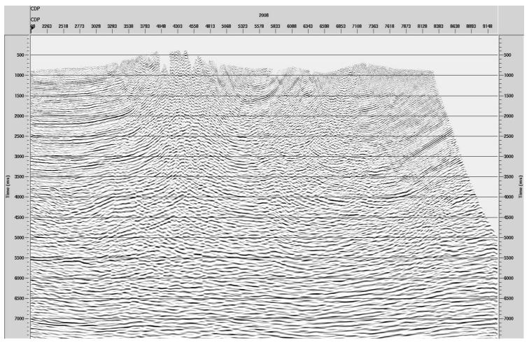
Fig. 1 Regional 2D Line. (a) Note the difference in the fold of coverage values (CMP_Fold_Geometry) due to having a smaller source station interval for low S/N ratio areas. (b) Final Stack (W-E direction). The recording was done using a roll-on on the west side and a full spread on the east side of the line.
3D Fold Parameters
The inline and xline fold formulas are based on inline and xline patch dimensions and for an orthogonal layout (Coardsen 2000):
- Inline fold = # of live channels in one RL × (RI / 2) / SLI
- Xline fold = NRL / 2
- Total Fold 3D = Inline fold × Xline fold
Where:
- RL = Receiver Line
- RI = Receiver interval
- SLI = Source Line interval
- NRL = Number of receiver lines in the recording patch (always an even number).
The formulas also assume that all the source points are within the recording patch and that the bin size remains constant. The Inline and Xline fold values must be integers for a smooth total 3D fold.
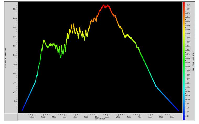
Fig. 2 Example of a smooth 3D Total fold (Total fold = 50. Inline fold = 10 and Xline fold = 5).
Recording Geometry Example
For the smooth 3D Total fold example displayed above, the physical recording geometry metrics break down as follows:
- 80 live channels per RL
- 20 RL in the recording patch
- RI = 25 m
- SLI = 200 m
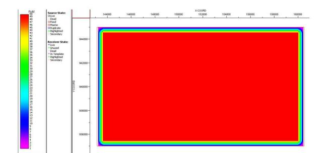
Fig. 3 Comprehensive diagnostic matrix visualization displaying localized inline and xline channel assignment sweeps matching the core execution values.