
2.3 Vibroseis Principles & Signal Processing
What is a Vibroseis?
A Vibroseis ( or vibrator unit ) is a seismic source which produces seismic energy (mostly P(compressional) wave) with control amplitudes and phase in a specific frequency range. It is a seismic source of high energy but low power. This feature makes the Vibroseis the ideal seismic source to work near infrastructures or even on pavement.
How does it work?
In very basic words, it is a hydraulic-servomechanism system mounted in an all-terrain vehicle , which reproduces a mechanical vibration (sweep) previously defined digitally.
Elements of the Vibroseis.
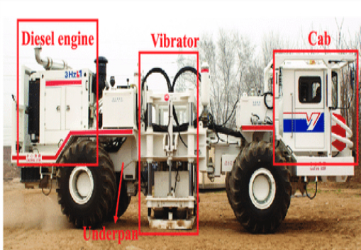
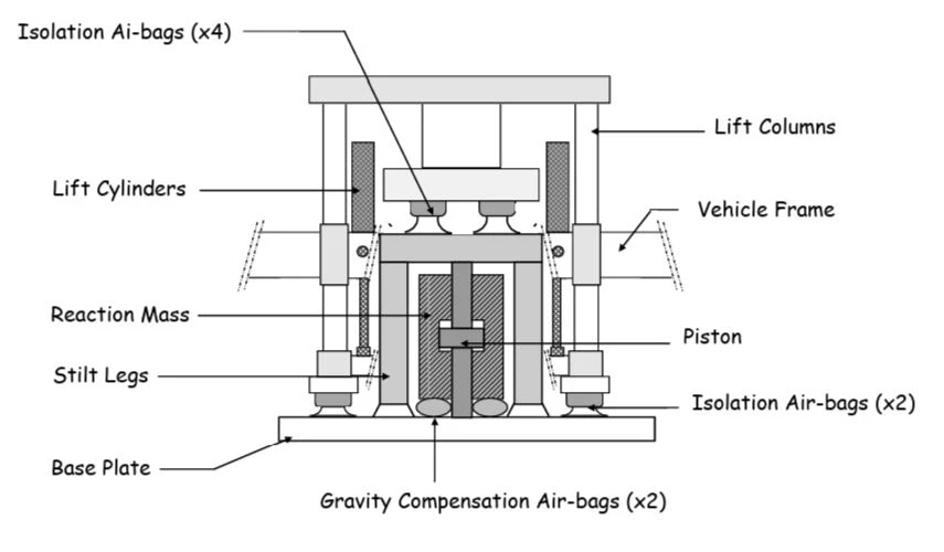
Figure 1. Elements of the Vibroseis. Vibrator ( shaker ) description.
The vibrator uses high-pressure hydraulic oil, controlled by a servo valve, to move a heavy reaction mass up and down; Newton’s Third Law converts that motion into force on the baseplate, which transmits seismic energy into the Earth while accelerometers continuously provide feedback, so the actual motion follows the desire sweep.
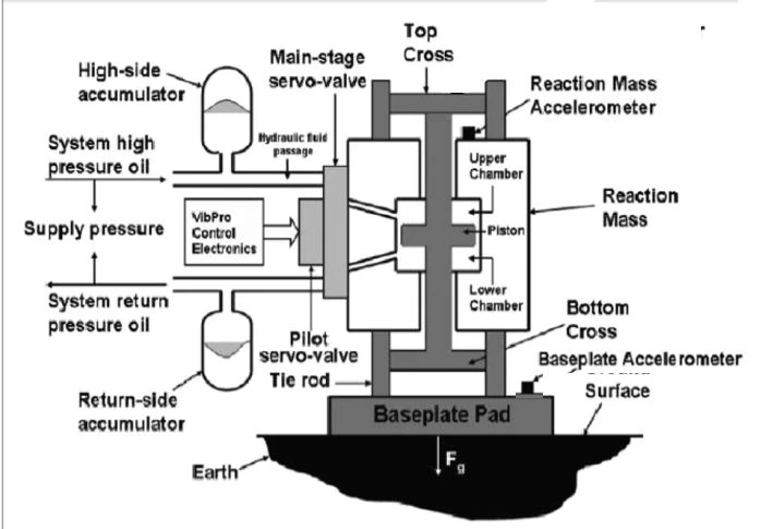
Figure 2. Diagram of the vibrator mechanism.
Elements of the vibro mechanism:
- 1.- Hydraulic system ( The source of the vibrator energy ): the engine drives hydraulic pumps that generate high pressure oil. Hydraulic oil is the main energy source used to move the reaction mass.
- 2.- Accumulators (Hydraulic batteries): the high-side and return-side accumulators store hydraulic energy , smooth pressure fluctuations, and provide the large instantaneous flow rates needed during high frequency sweeps.
- 3.- Pilot Servo Valve (First amplifier): The Pilot Servo valve converts a small electronic command into a hydraulic control action. It acts like the steering wheel for the larger hydraulic system.
- 4.- Main-Stage Servo Valve ( one of the critical components): the main servo valve directs high-pressure oil to either the upper or lower chamber of the hydraulic actuator inside the reaction mass. It determines the motion of the reaction mass.
- 5.- LVDT ( Linear variable differential transformer ): It is a very accurate linear displacement sensor. A LVDT on the mass gives instantaneous position of the reaction mass respect of the baseplate, and a LVDT on the valve gives the real position of the spool inside the servo valve.
- 6.- Piston ( Inside the reaction mass ). Here is the pressure to force conversion: Hydraulic pressure acting on the piston creates a force ( F = P x A ), where the force is equal to the pressure multiplied by piston area. ( Pascal Law ).
- 7.- Reaction Mass ( The moving weight ): The reaction mass is a heavy moving element ( e.g. Mass of the reaction mass is 4700 kg on Sercel Nomad 65 Neo vibrator ), that oscillates up and down according to the sweep command generated by the vibrator electronic controller (VEC).
- 8.- Baseplate ( Ground Coupling ): When the reaction mass accelerates, an equal and opposite force is generated ( Newton’s third law ). This force is transmitted to the baseplate and ultimately into the surface ground. A good baseplate coupling improves the seismic signal quality and reduces the phase and harmonic distortion.
- 9.- Accelerometers ( The feedback control ): Reaction-mass and baseplate accelerometers measure the actual motion. The VEC compares desire motion ( sweep ) with the actual motion and continuously corrects the servo valve, forming a closed-loop servo system.
- 10.- Vibrator Electronic Control- VEC (The Brain): The controller generates the desired sweep and continuously calculates how the vibrator mechanisms should move or act at every instant.
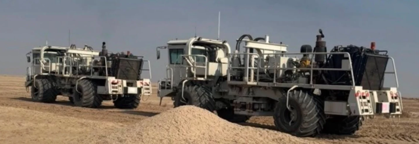
Figure 3. Sercel Nomad 65-Neo Vibrator.[cite: 1]
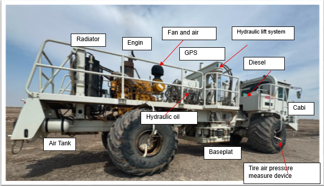
Figure 4. Some elements of the Sercel Nomad 65-Neo Vibrator.[cite: 1]
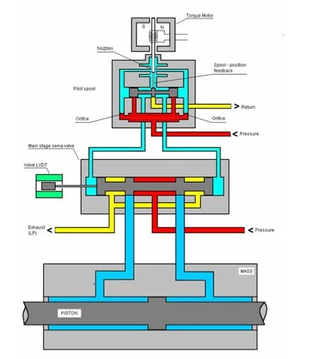
Figure 5. Diagram of Typical servo valve. Toque motor and servo hydraulic valve. The vibrator electronics continuously monitor the ground force and adjust the toque motor current to keep the amplitude and phase of the ground force signal as close as possible to the reference sweep. (Sercel.com) and (Verif-i.com).[cite: 1]
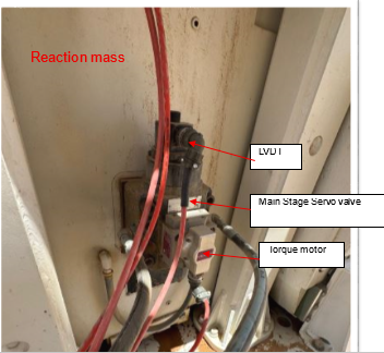
Figure 6. Torque Motor and Main Servo valve.
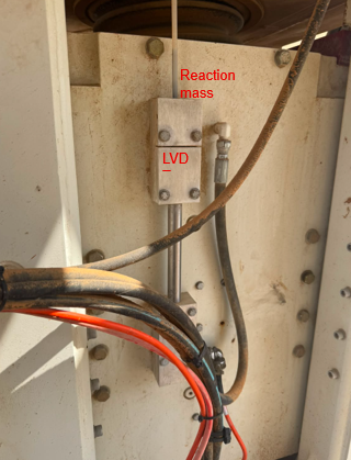
Figure 7. LVDT of the reaction mass.
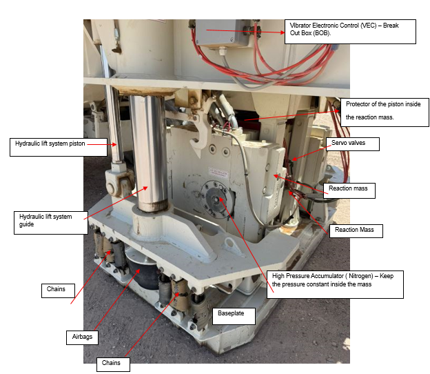
Figure 8. Elements of the vibrator.
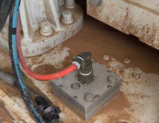
Figure 9. Accelerometer on the baseplate.
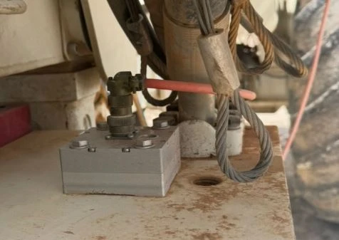
Figure 10. Accelerometer on the reaction mass.
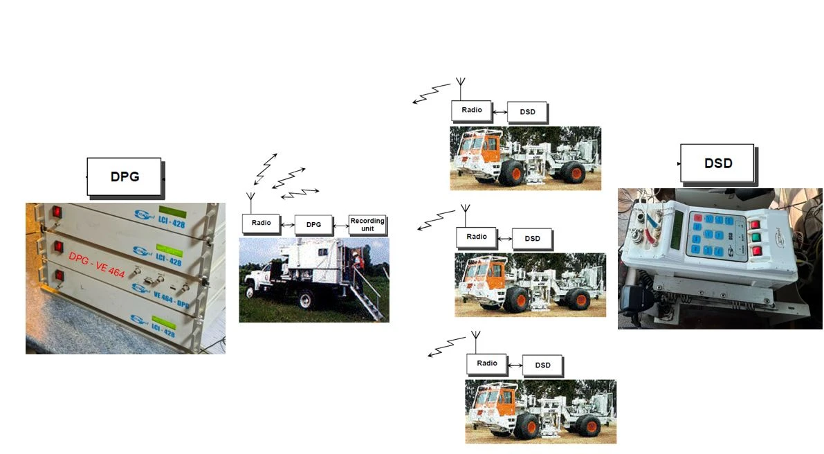
Figure 14. Sercel VE-464 Vibrator Control System. The DPG ( Digital Pilot Generator ) is installed on the recording truck and connected with the seismic recording system (Sercel 428 XL). It communicates via Radio with the DSD ( Digital Servo Drive ) installed on each vibrator.[cite: 1]
The Digital Pilot Generator (DPG):
- It generates Pilot Sweep. The reference signal to do the cross correlation.[cite: 1]
- It loads all parameters of the sweep into the DSD via radio.[cite: 1]
- It synchronized the DSD (T0 command): prior to each acquisition the DPG sends a synchronization code to each DSD to start the sweep.[cite: 1]
- DPG stores all QC results received from DSD via radio.[cite: 1]
The Digital Servo Drive (DSD):
- It is mounted on each vibrator unit.[cite: 1]
- It receives and stores the sweep parameters, sweep selection and T0 command.[cite: 1]
- Controls the actuator and the baseplate motion to minimize ground force signal phase and distortion errors.[cite: 1]
- It controls the reaction mass and baseplate motions, DSD relies on four sensors: 1) accelerometer on the reaction mass, 2) accelerometer on the baseplate, 3) LVDT on the reaction mass and 4) LVDT on the Servo valve ( Spool ).[cite: 1]
- Compute Real Time QC results, generate status and send the information to the DPG by radio.[cite: 1]
In Summary: DSD generates a local sweep reference ( sweep on each vibrator ), continuously control of the vibrator shaker’s motion and perform real time QC of the Ground Force Signal of the vibrator.[cite: 1]
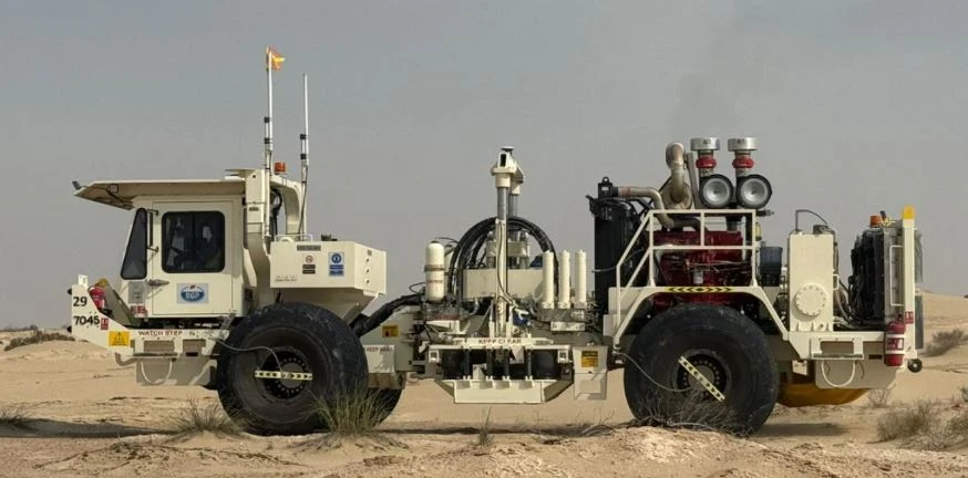
Figure 15. Vibrator INOVA AVH-V-480.
Quality control of the Vibrators.
There are several files and tests that help to evaluate the performance of the vibrator during seismic data recording production, their configuration and their fidelity to reproduce (mechanically) the desired sweep with phase and amplitude within specifications and minimum harmonic distortions.
1) Get-DSD File QC
Sercel DSD produces a file with all vibrator configuration values and measurements from some mechanical elements for quality control. It is very important to check that all vibrators in production are set up with the same configuration values. This file is sent to DPG by DSD by radio.
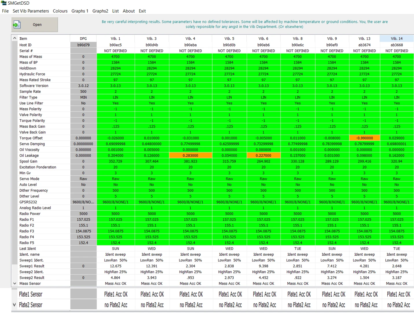
Figure 16 . An example of a Get-DSD file. The software SMGetDSD (seismatter.com) is able to visualize and make QC of the values per vibrator. Green color =Ok. Orange = warning. Red= error. Correct defined values such as mass polarity, valve polarity and torque polarity have paramount importance.
2) Similarity tests
There are some tests to evaluate how similar the Pilot Sweep ( created by DPG ) and the physical shake (sweep) created by the Vibrator ( Ground Force ) are each other. There are two types of similarity tests: by cable ( hardwire ) and by radio.
Hardwire Similary test: It is usually done on a monthly basis, and it uses 4 special cables which are connected from the DSD to the recording Instrument.
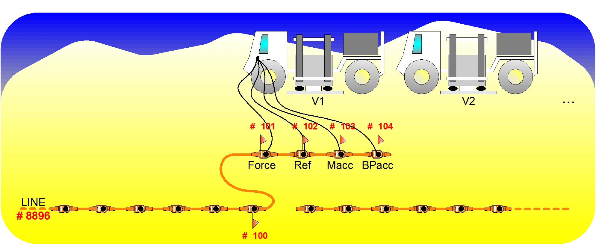
Figure 16. Hardwire Similary Test Diagram. From this test We have five channel information. Channel 1: Pilot sweep (DPG), Channel 2: Reference (Vib) sweep (DSD), Channel 3: Ground Force (DSD), Channel 4: Mass accelerometer (DSD), Channel 5: Baseplate accelerometer (DSD).

Figure 16. Hardwire Similary Test.
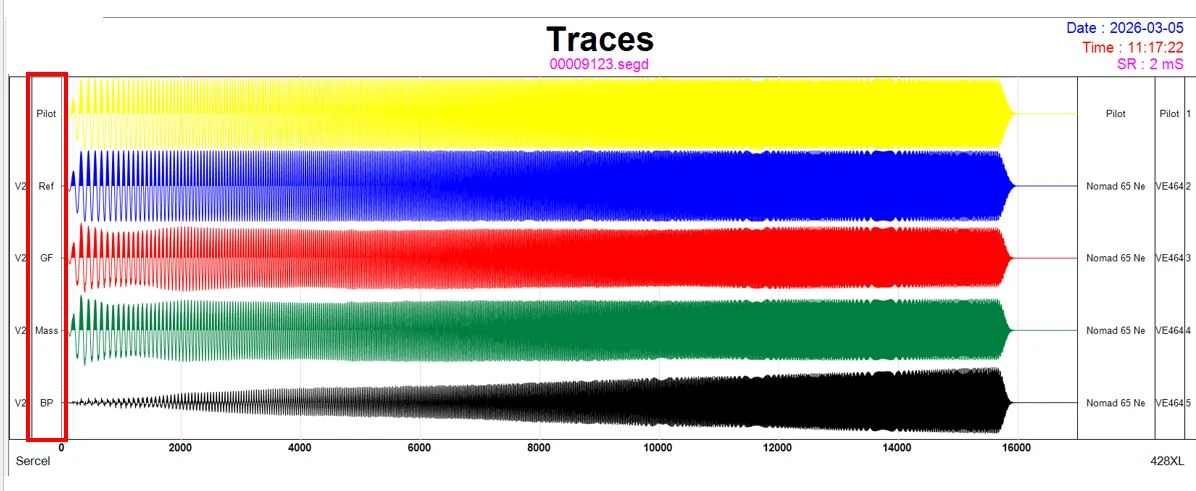
Figure 17. Hardwire Similary Test Camera (the five channel display)
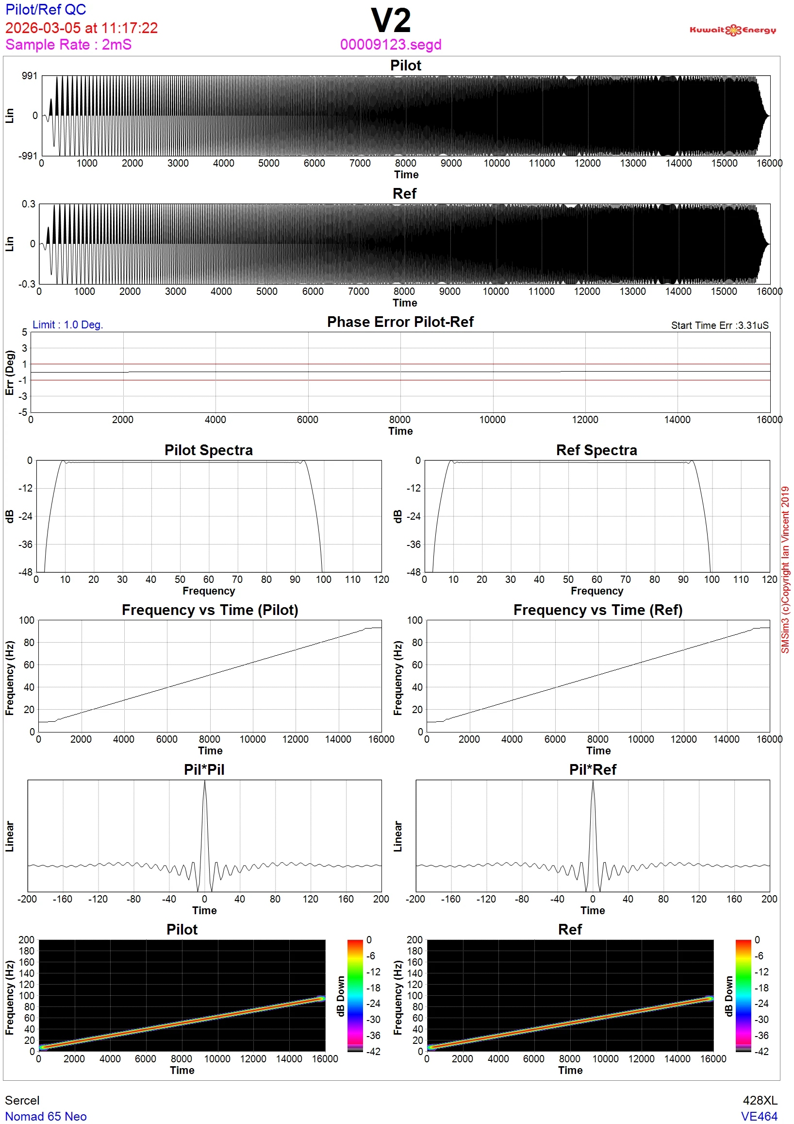
Figure 18. QC between the Pilot Sweep (DPG) and Reference Sweep (DSD). They must be identical. (SMSIM3- Seismatter.com)
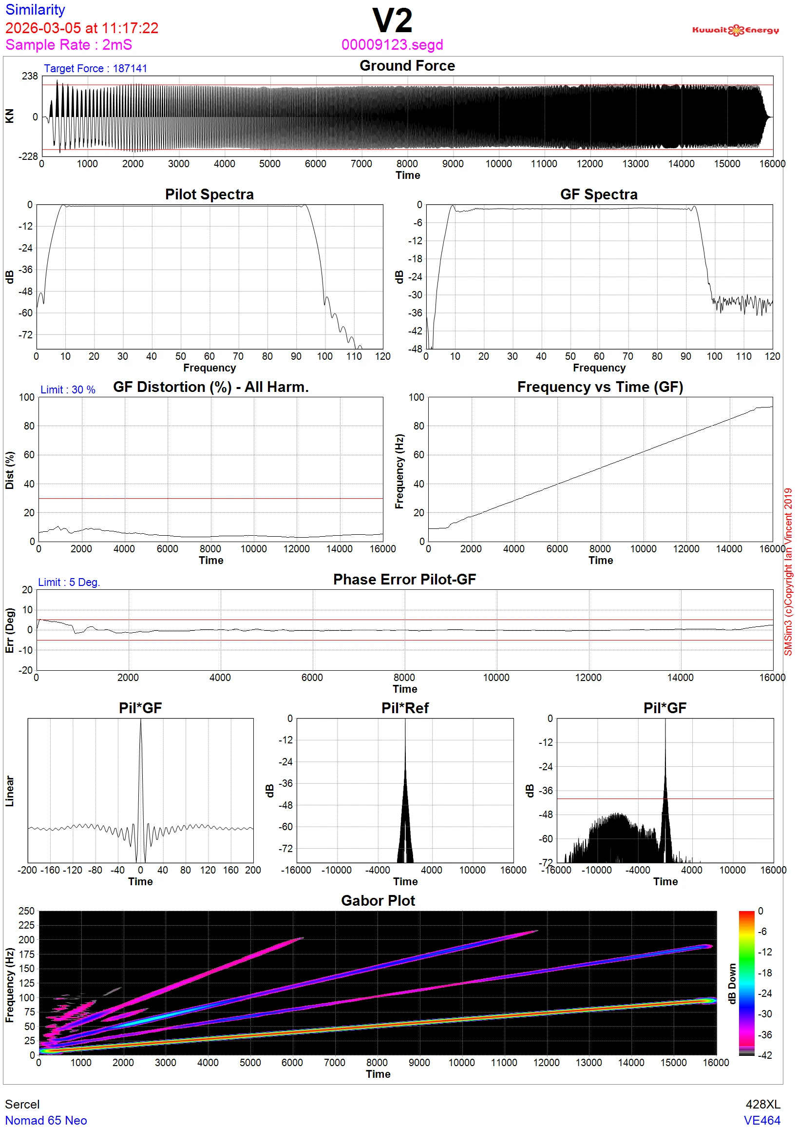
Figure 19. QC between the Pilot Sweep (DPG) and Ground Force - GF (DSD). The differences must be inside the tolerances (Red lines). (SMSIM3- Seismatter.com)
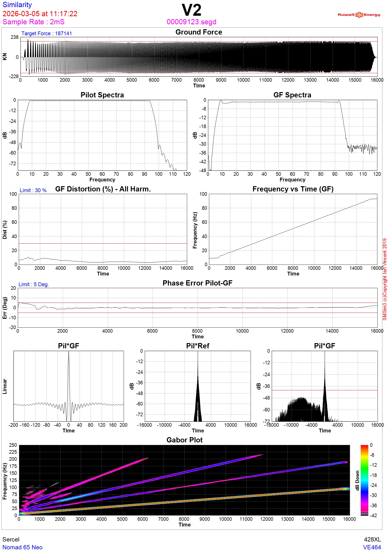
Figure 20. QC for Ground Force (GF) Distortion. (SMSIM3- Seismatter.com)
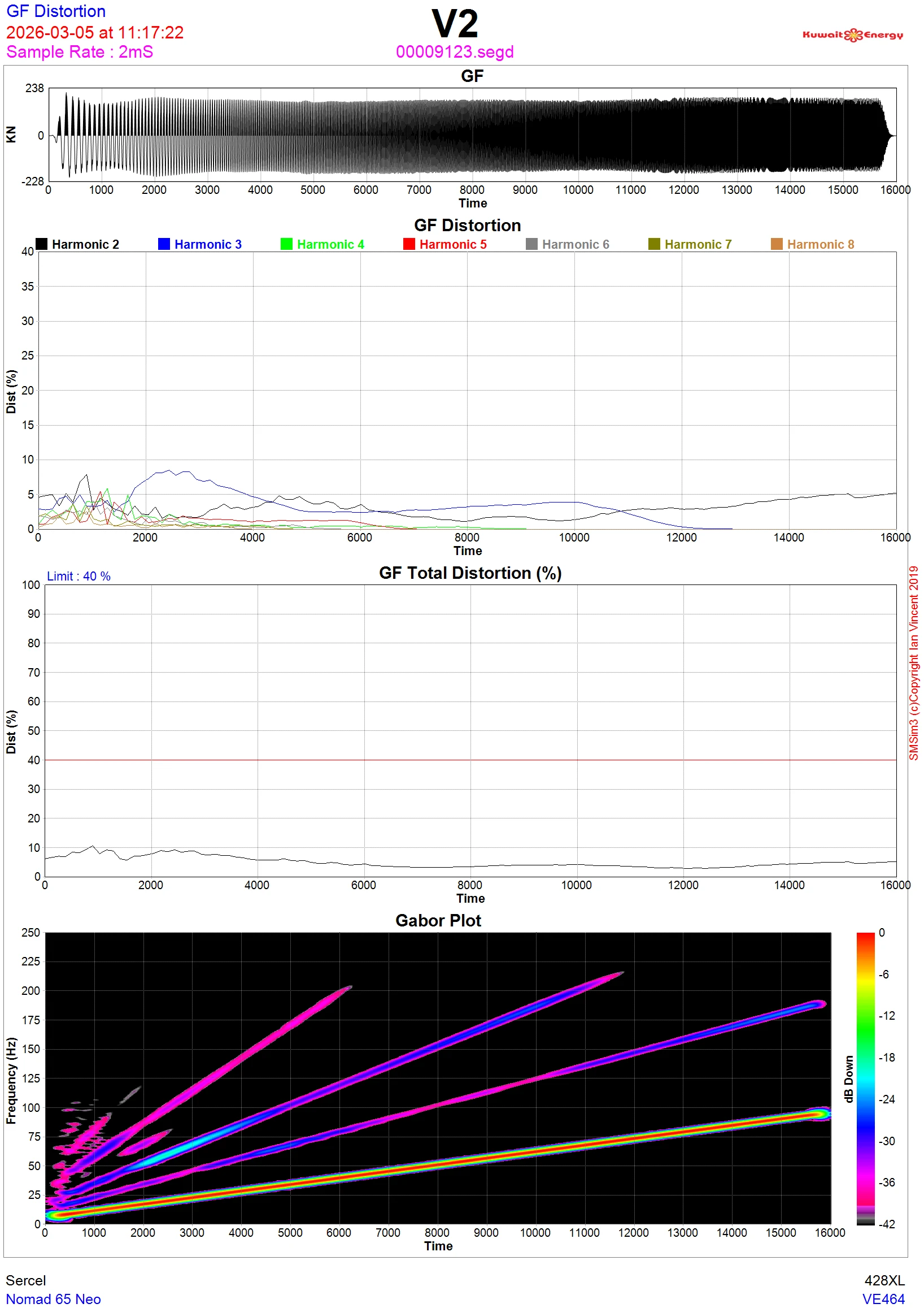
Figure 21. QC for Ground Force (GF) distortion using an Independent Force Calculation. (This is a calculation done using the outputs of the vibro accelerometers rather than just relying on the calculated GF from the DSD. (Seismatter.com). Results should be the same as on Figure.19.
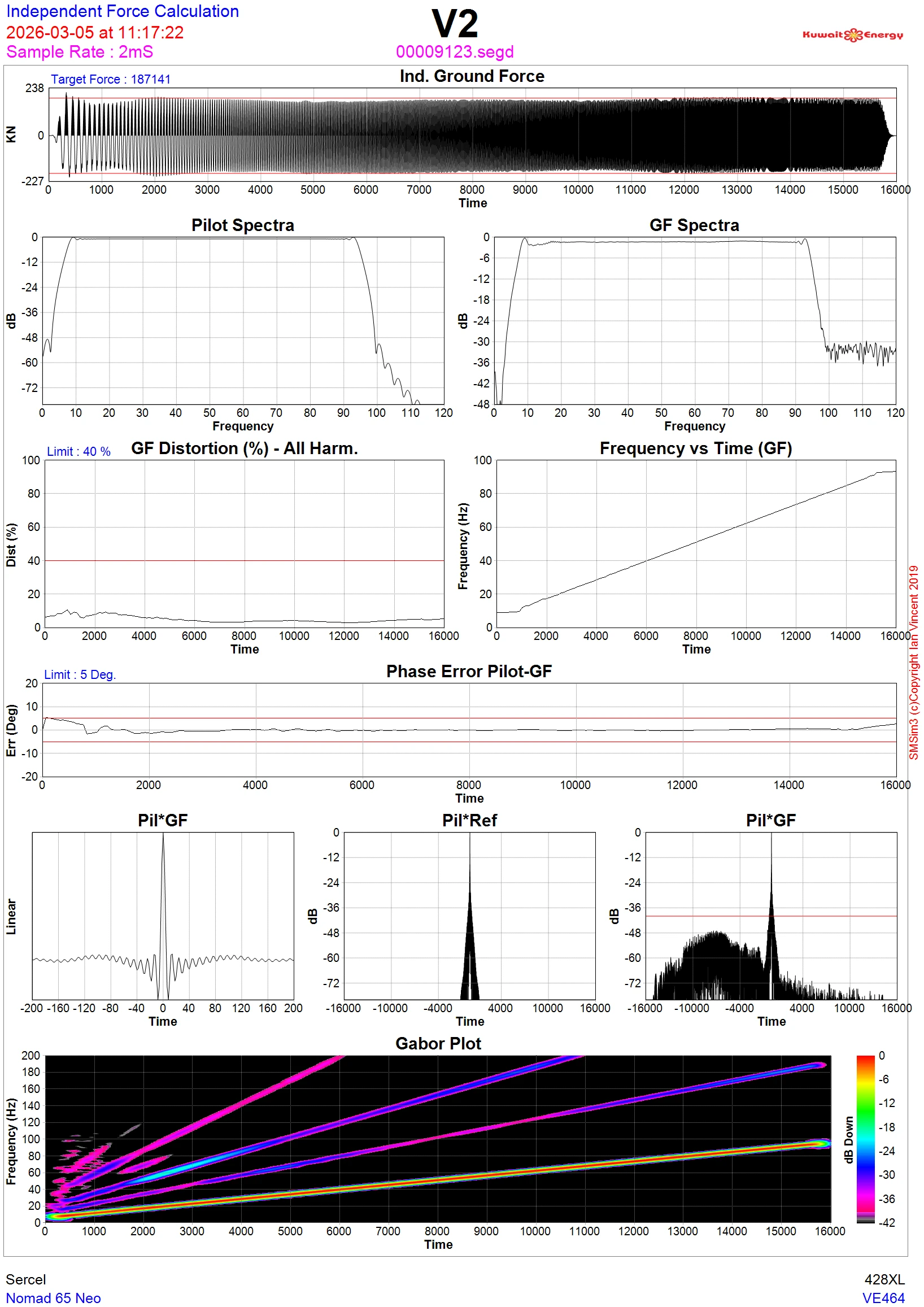
Figure 22. QC for the defined Taper (in ms). (Start and end tapers of the sweep).
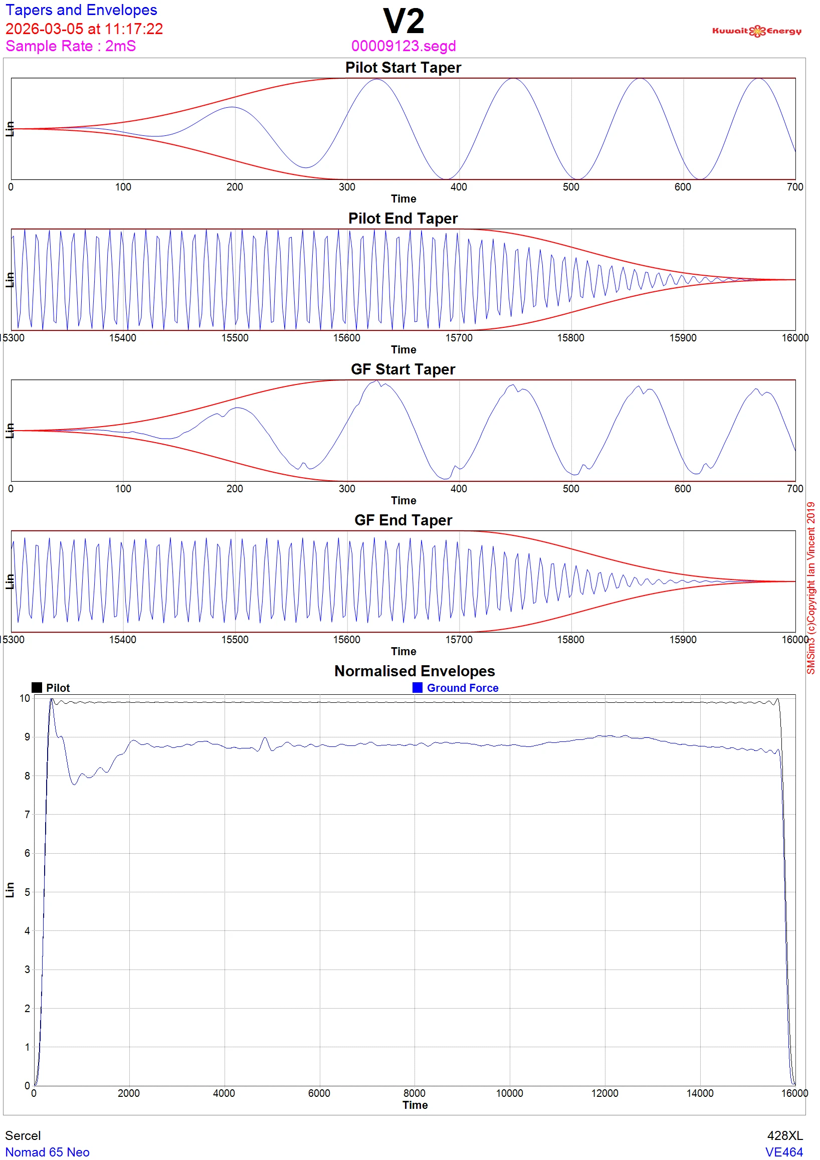
Figure 23. QC Mass – Baseplate Relationship QC.
Remarks:
On this example , the sweep was defined as follows:
- - Sweep length: 16 seconds.
- - Sweep type: Linear – Up-sweep.
- - Taper: 350 ms.
- - Drive: 75%.
- - Frequency range: 6-96 Hz ( 4 Octaves ).
- - Listening time: 6 seconds.
- - Record length ( correlated ): 6 seconds.
From Figure. 18, you can see the QC comparison between Pilot sweep and Reference sweep. Their correlation and autocorrelation are identical. (They want to be a Dirac Delta). No phase differences, No harmonic energies in the Gabor Plot, a linear up-sweep frequency distribution and clean amplitude spectrum. Also, it indicates the start time error of 3.3 microseconds.
The start time error calculation is based on the phase error between the reference sweep and ground force. A FFT is calculated for both reference sweep and ground force. Thus, we will get the amplitude and phase values for each frequency component (bin) on the sweep. A least square ( regression ) is performed to determine start time error. (Seismatter.com).
The Testify ( Verif-i.com ), calculates the start time error in a similar way but it is used the cross correlation of reference sweep and ground force against the autocorrelation of the reference sweep. (Seismatter.com).
In any case, if the maximum phase error between Reference and GF is inside the tolerance ( it is usually 5 degrees). The start time error will be ok. (Seismatter.com).
Figure 19 is the tough real life. It is the QC between the Pilot Sweep (DPG) and the Ground Force calculated by DSD using accelerometer measurements. It is a real indicator of the quality of the sweep ( shaking ) introduced to the ground through the baseplate. The key is to be inside the tolerances ( red lines ).
Figure. 20. There are more details on the Ground Force distortion. (even and odd harmonics analysis ).
Figure. 22. QC for the defined Taper (in ms). For this example, the taper value is 350 ms. The Taper ( a square cosine function) helps vibrator (shaking) performance at the beginning/end of the sweep and minimize the side lobes on the correlation, minimize the harmonic creation, stabilize the Gibb effect and help the vibrator on de coupling baseplate-ground.
Figure. 23. QC Reaction Mass – Baseplate Relationship QC. This QC checks how efficiently the motion from the reaction mass becomes useful seismic force into the ground ( Baseplate ).
The oscillation from the reaction-mass ( MASS ) follows the desired sweep. The velocity is more or less constant along the sweep. Keep in mind that lower frequencies require a bigger mass stroke than higher frequencies.
The oscillation from the baseplate ( BP ) shows the actual energy transmission to the ground. The transmitted energy for low frequencies is not efficient. ( the reaction mass is moving a lot , but the ground is not moving proportionally ). One of the reasons is the poor coupling at the beginning of the sweep. At higher frequencies the coupling becomes more efficient, and more force is converted into BP motion. ( Smoothly, monotonic and and stable-linear increase of Phase-Mass-BP and Transfer (BP acc/Mass acc) function graph, it is what we want for a healthy vibrator.
At low frequency: acceleration is low, mass stroke must increase then more oil flow is required. This is why distortion increases at low frequency, harmonics appear and the energy transfer becomes less efficient.
Vibrator Polarity
When we talk about “vibrator” polarity, we are actually referring to the polarity of the vibrator (feedback) accelerometers.
We want to check if the baseplate accelerometer (feedback) polarity is correct relative to the expected baseplate-motion and SEG polarity convention. (Sercel Vibrators).
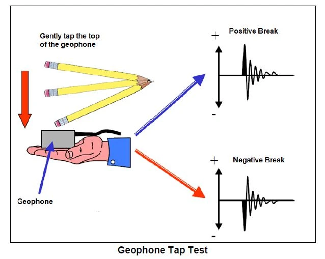
Figure 24. Tap test for a geophone. The SEG Polarity Convention established that for a downward impulsive (case) motion (the red arrow) result in a positive kick (break) on a monitor record. (the blue arrow). (Verif-i.com).
For vibrators, the pulse test is the equivalence to the tap test for geophones.
Vibrator accelerometers are bolted to structures of the vibrator ( mass and baseplate ) and cannot easily be removed for a tap test. However, a pulse sweep can be used to verify the accelerometer polarity.
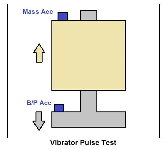
Figure 25. Vibrator Pulse Test. When the pulse is executed, the mass is initially driven upwards and the baseplate downwards. This is equivalent to tapping the top of the baseplate accelerometer and tapping the bottom of the mass accelerometer. (Verif-i.com).
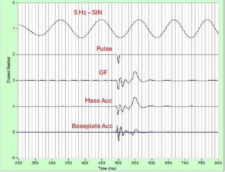
Figure 25. Vibrator Pulse Test. The graph shows the result of a vibrator pulse test on a system ( accelerometers ) complying with the SEG Polarity convention. (Verif-i.com):
- The baseplate is driven downwards, which is equivalent to a tap on the top of the accelerometer, and it breaks positive.
- The mass is driven upwards, which is equivalent to a tap on the bottom of the accelerometer, and it breaks negative.
- The ground force signal is dominated by the mass and breaks negative.
- The reference is in phase with the ground force and breaks negative.
Remark: The vibrator accelerometers must have the same polarity convention as the seismic receivers. This ensures that the correlator preserves the correct polarity of the seismic data after correlation.
A Funny Test
The most common sweep type used is the (linear) up-sweep. The main reason is avoiding the amplitudes of the harmonics to be on the positive side of the correlation (and then producing noise in the correlated seismic data). In an up-sweep the amplitudes of the harmonics will be in the negative side of the cross-correlation.
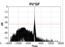
Figure 24 . Cross- correlation of the up-sweep pilot and Ground Force . ( From figure 21 ).
So, what happens if made a similarity test for a down-sweep ( From 90 to 10 Hz ) ?
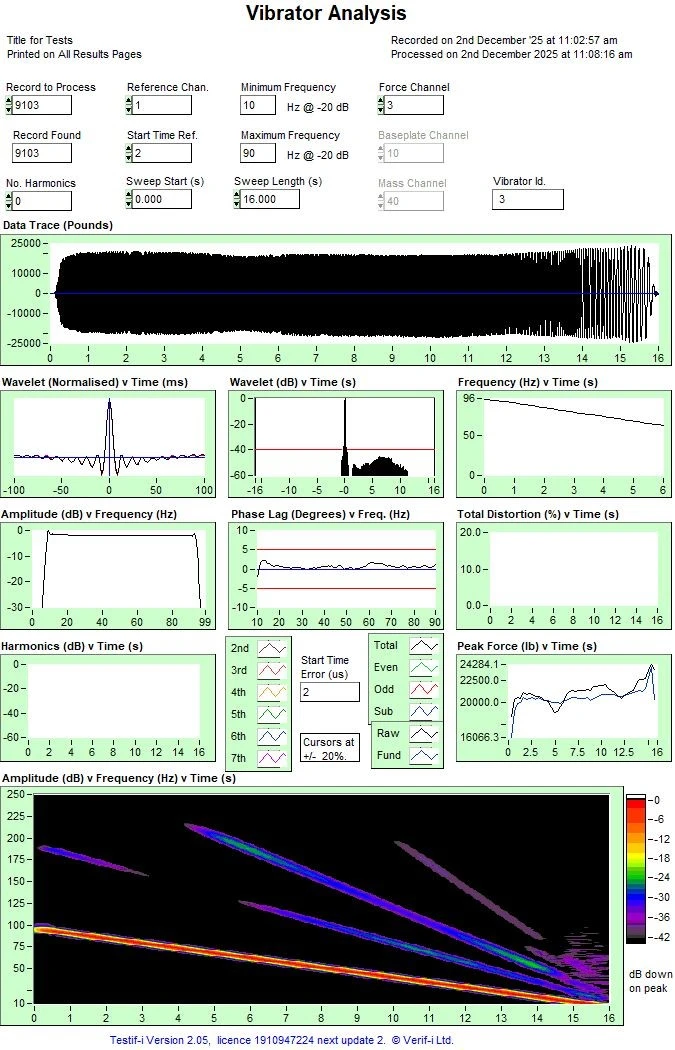
Figure 25a. A funny test. Similary Test for a down-sweep showing harmonic amplitudes on the positive side of the cross correlation
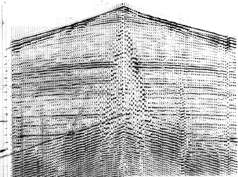
Figure 25b. A down sweep shot gather shows the harmonic noise in the correlated seismic data. Modified from Mustagh Resources (mustagh.com).
QC of vibrator performance during recording production
There are several files which help to evaluate the vibrator performance during production. One of the main ones are the VAPS files. VAPS files are generated directly by Sercel recording systems and vibrator control electronics (e.g. VE464) as quality control (QC) logs for the seismic recording.
VAPS stands for Verbose Acquisition ParameterStatus. ( Verbose: highly detailed, comprehensive data):
- Vibrator Status: A single line/record is updated automatically for every individual vibrator after every sweep.
- Attributes Logged: They store phase errors, distortion percentages, force output levels, and critical GPS/RTK positioning data.
- Geographic Diagnostics: Because they pair parameter metrics with coordinates, geophysicists can plot VAPS data into geographical views to instantly isolate exactly where a vibrator underperformed on a survey line. (Verif-i.com).

Figure 26. A software header ( VASPDB3 – seismicmatter.com), showing the information can be displayed (scatter graph) for doing Q.C. of the vibro performance.
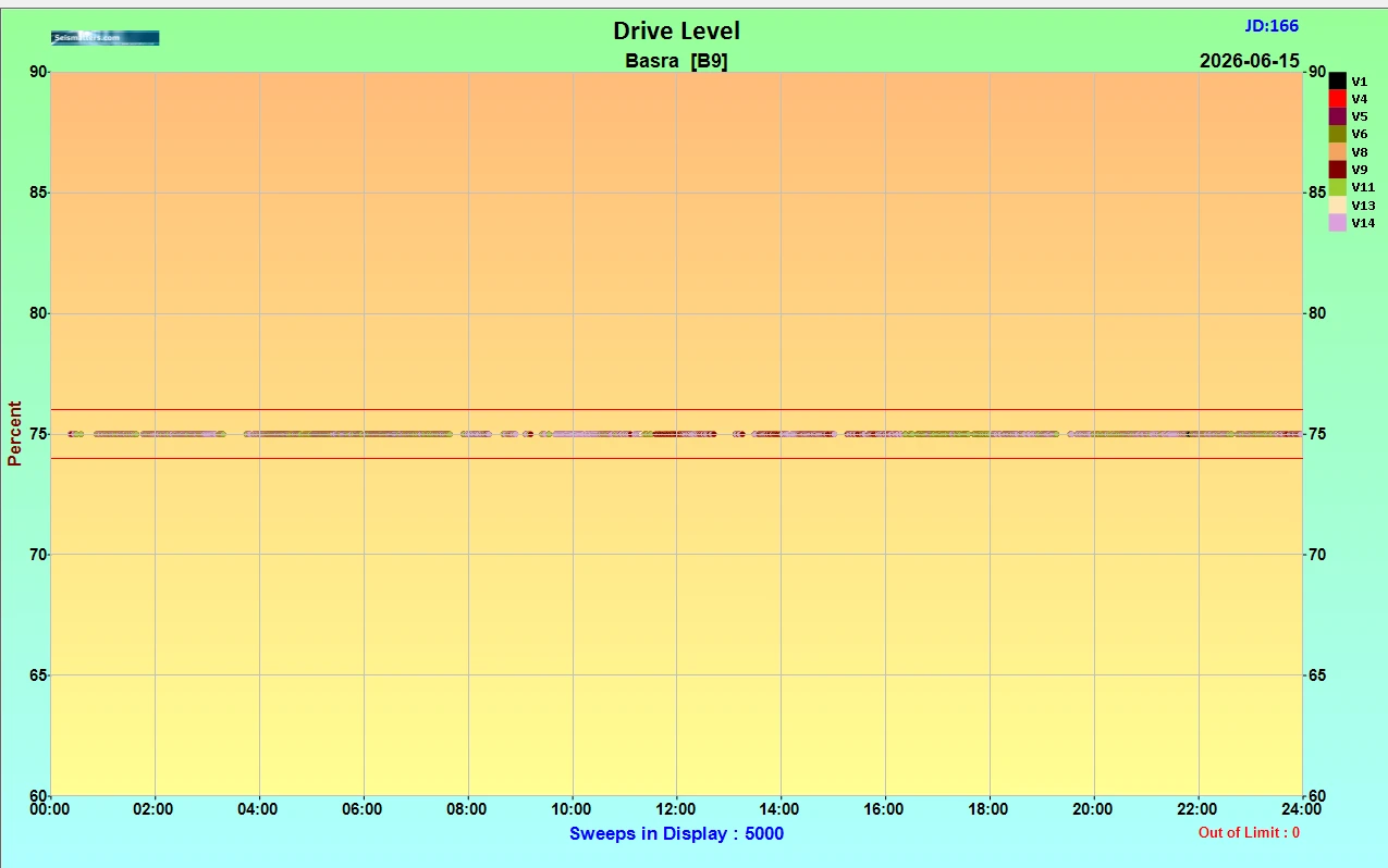
Figure 27. VAPS information: Drivel Level. ( For 5000 sweeps – All vibrators in production).
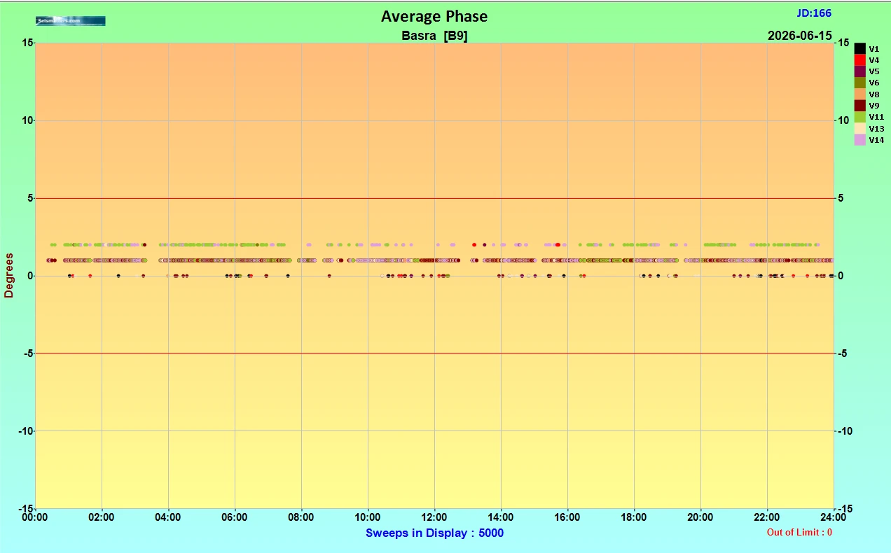
Figure 28. VAPS information: Average Phase. ( For 5000 sweeps – All vibrators in production). (Limits: -5 to 5 degrees).
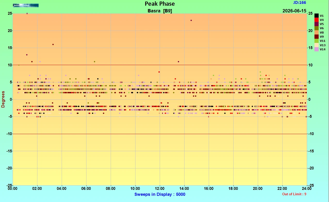
Figure 29. VAPS information: Peak Phase. ( For 5000 sweeps – All vibrators in production). (Limits: -10 to 10 degrees).
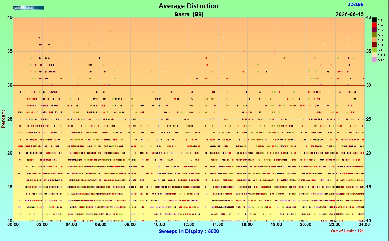
Figure 30. VAPS information: Average Distortion. ( For 5000 sweeps – All vibrators in production). (No more than 30 %).
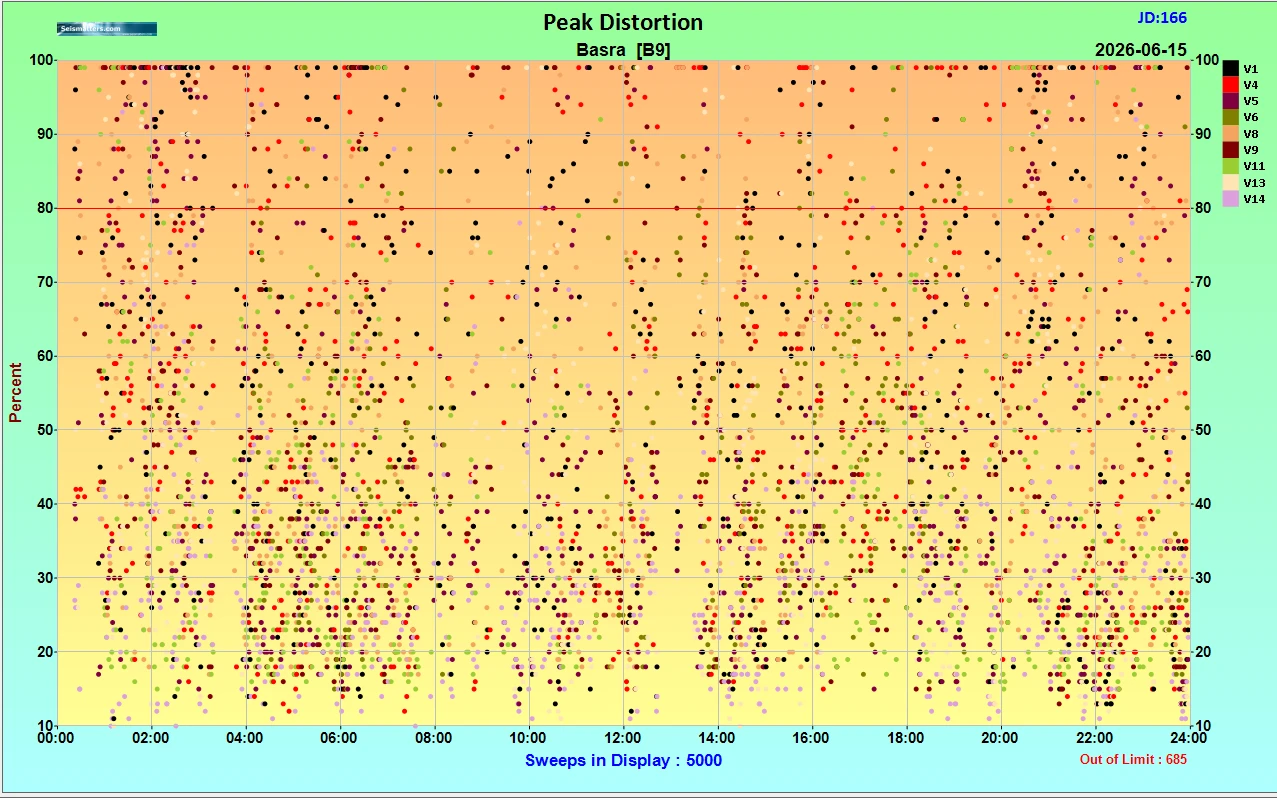
Figure 31. VAPS information: Peak Distortion. ( For 5000 sweeps – All vibrators in production). (No more than 80 %).
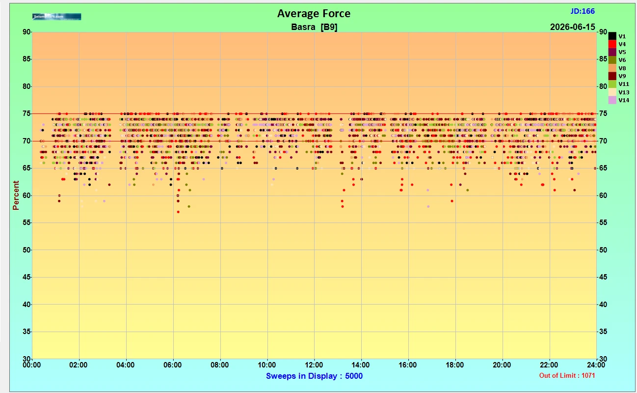
Figure 32. VAPS information: Average Force. ( For 5000 sweeps – All vibrators in production). (Range: 70-75 %).
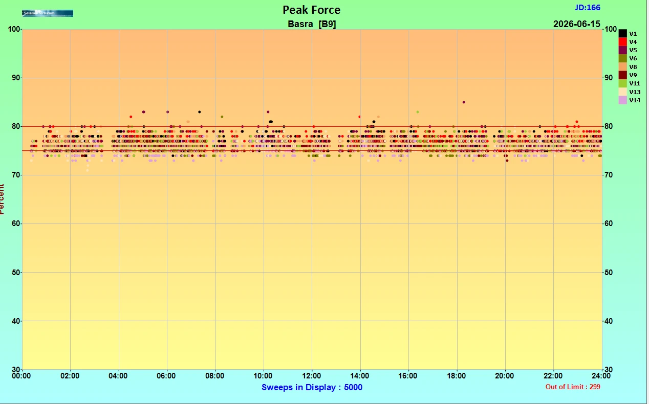
Figure 33. VAPS information: Peak Force. ( For 5000 sweeps – All vibrators in production). (Range: 75-80 %).
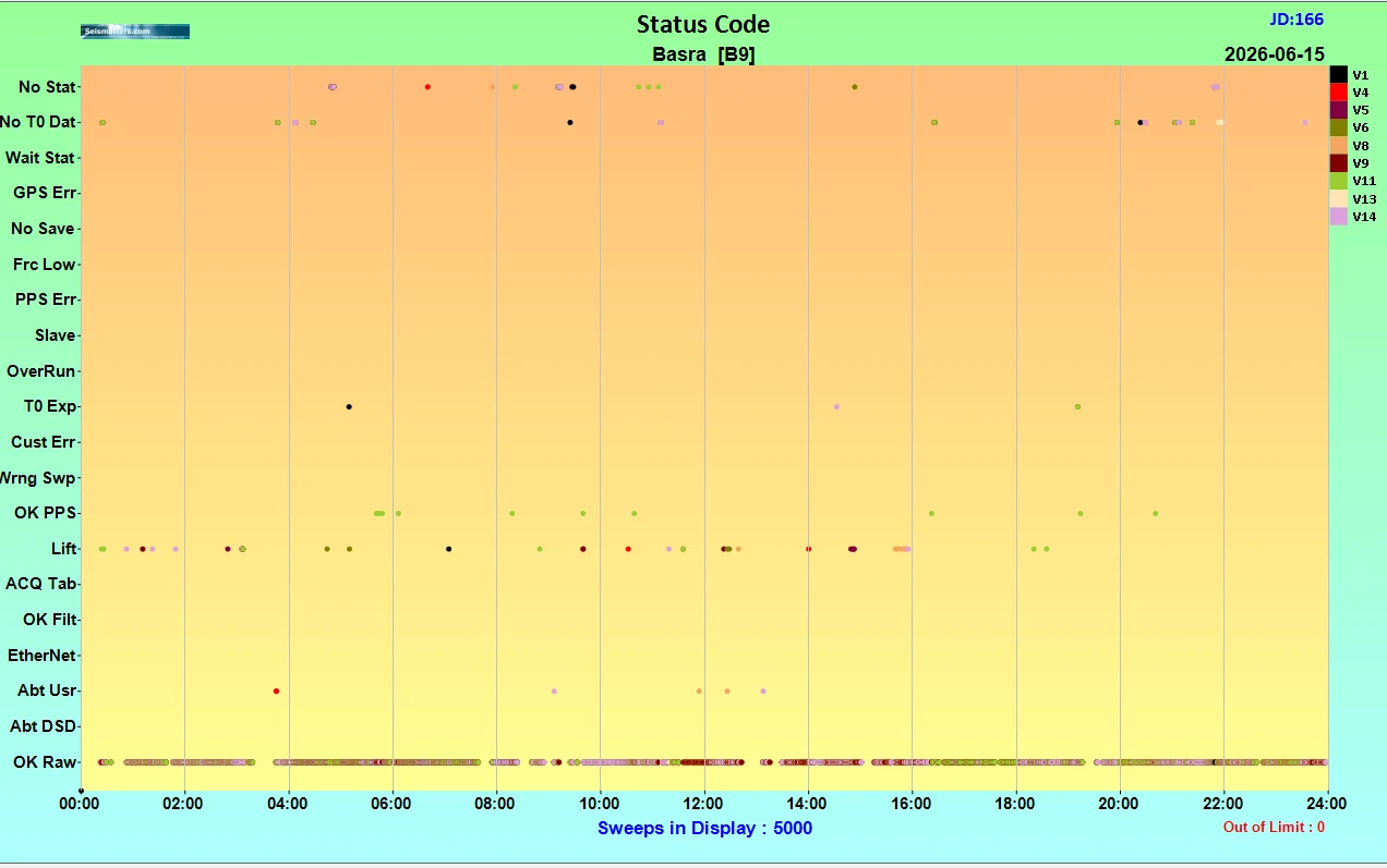
Figure 34. VAPS information: Status code for vibrator performance. ( For 5000 sweeps – All vibrators in production).
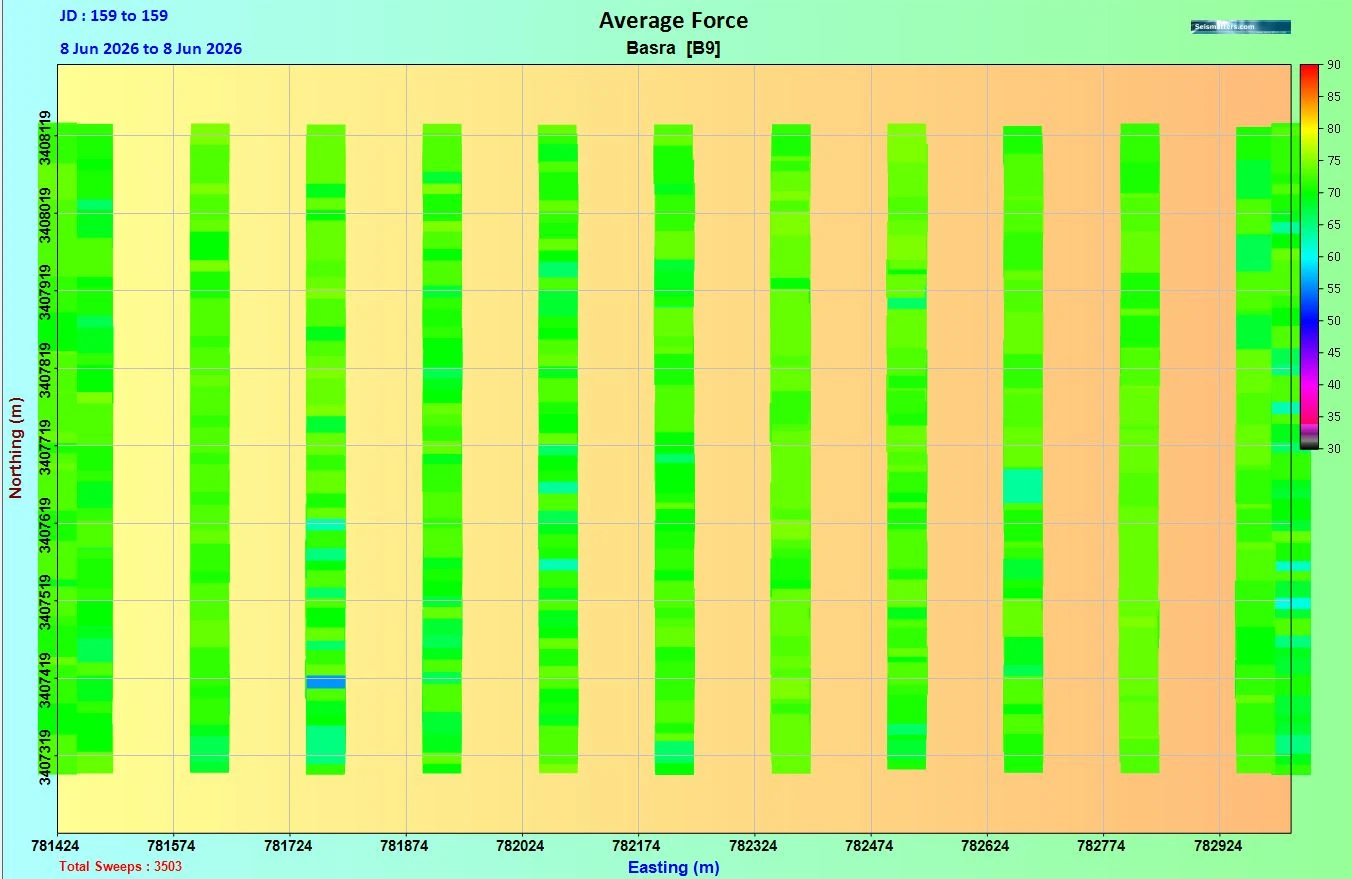
Figure 35. VAPS information: Average Force areal display.[cite: 1]
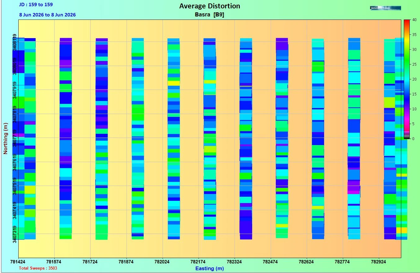
Figure 36. VAPS information: Average Force areal display.[cite: 1]
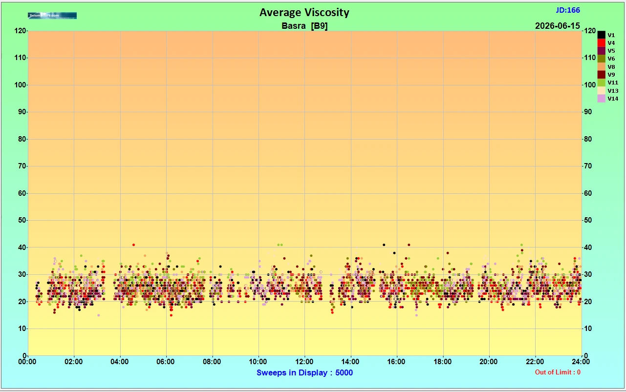
Figure 37. VAPS information: Average Viscosity.[cite: 1]
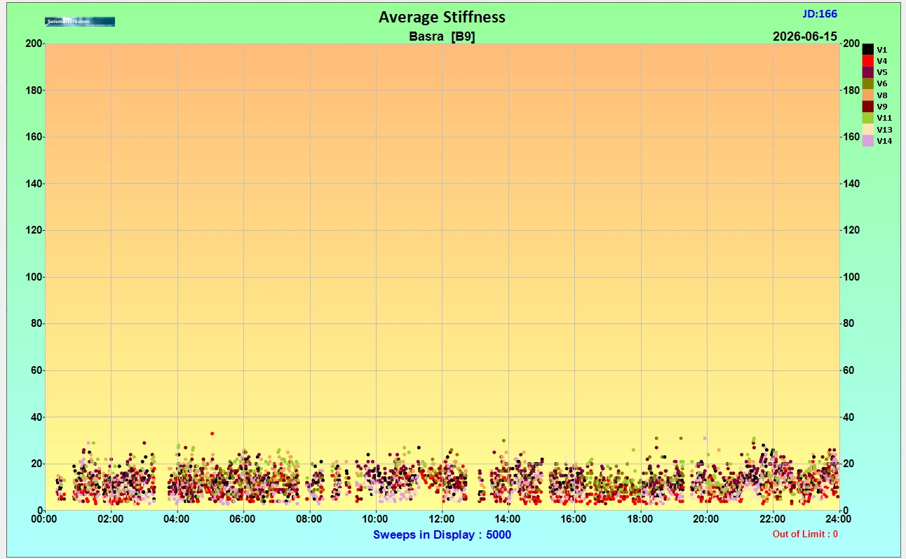
Figure 38. VAPS information: Average Stiffness.[cite: 1]
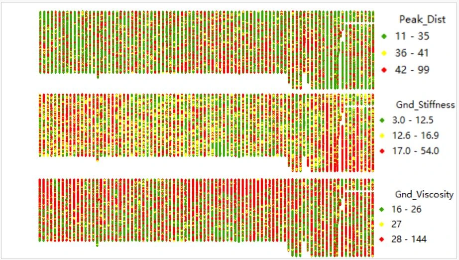
Figure 39. Analysis of the vibrator performance from VAPS data.[cite: 1]
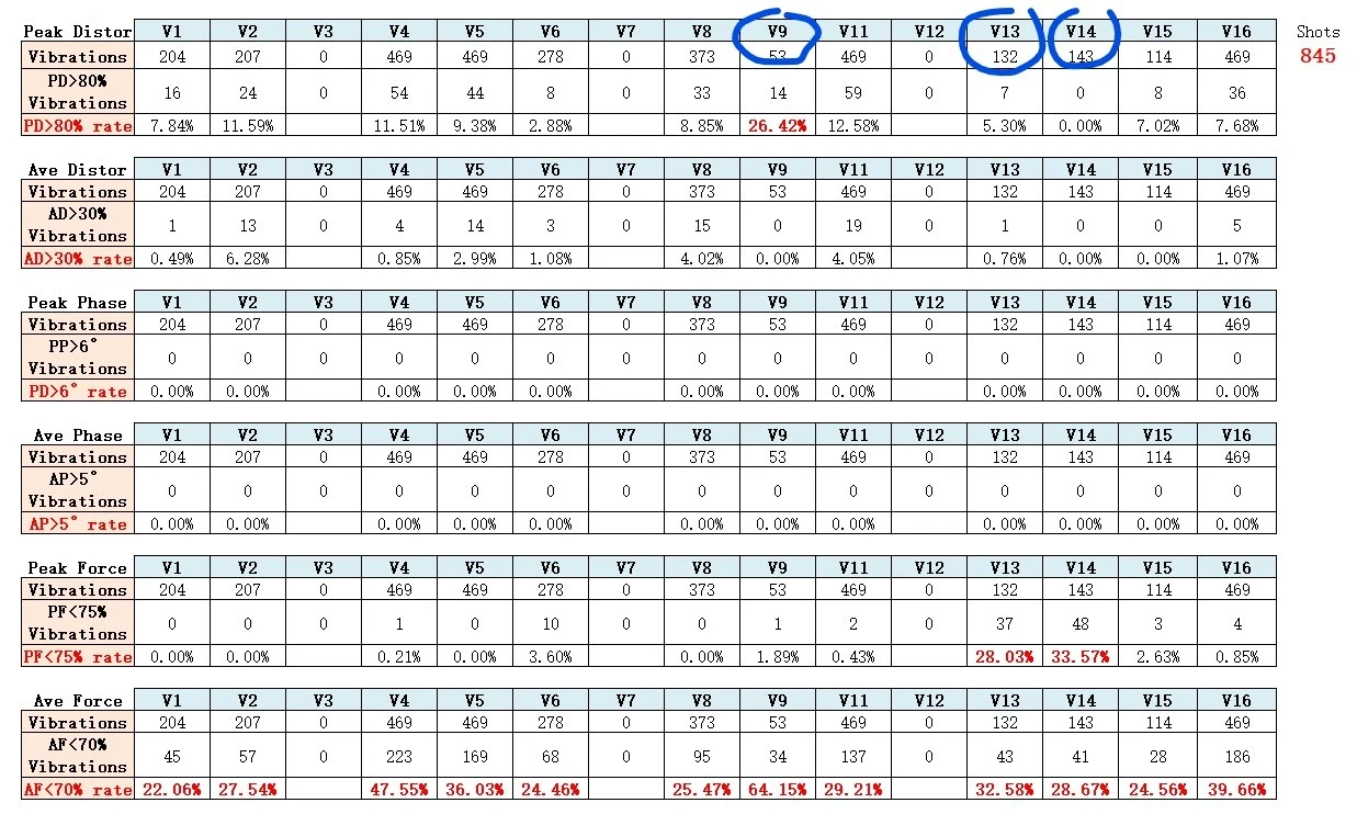
Figure 40. Analysis of relationship of high distortion with stiffness and viscosity of the ground.[cite: 1]
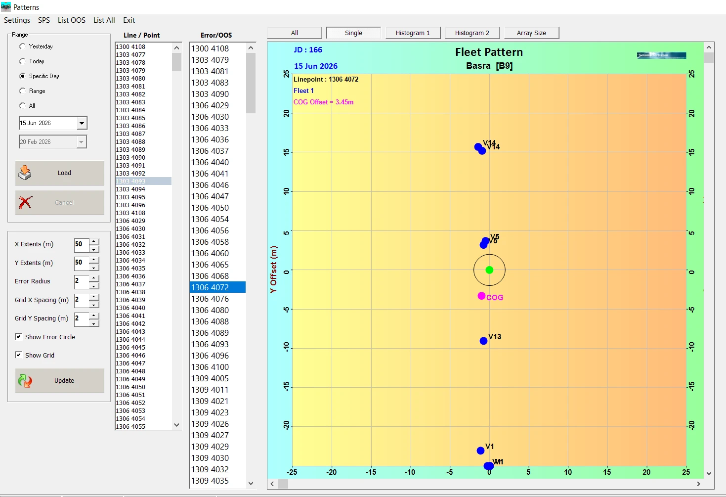
Figure 41. COG QC of the vibrator fleet. ( radio error: 2 meters – difference between the source station ( SPS - survey ) coordinates and the COG coordinates - vibrator fleet. They are calculated from the DGPS on each vibrator.[cite: 1]
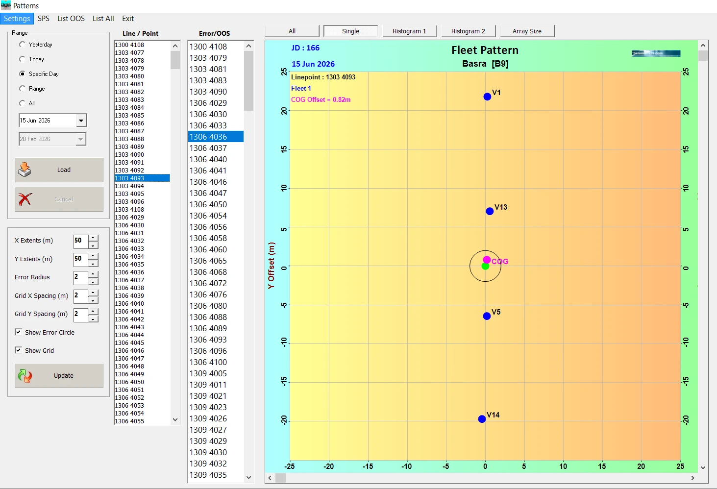
Figure 42. COG QC of the vibrator fleet. ( COG calculated coordinates inside 2-meter radio ).[cite: 1]
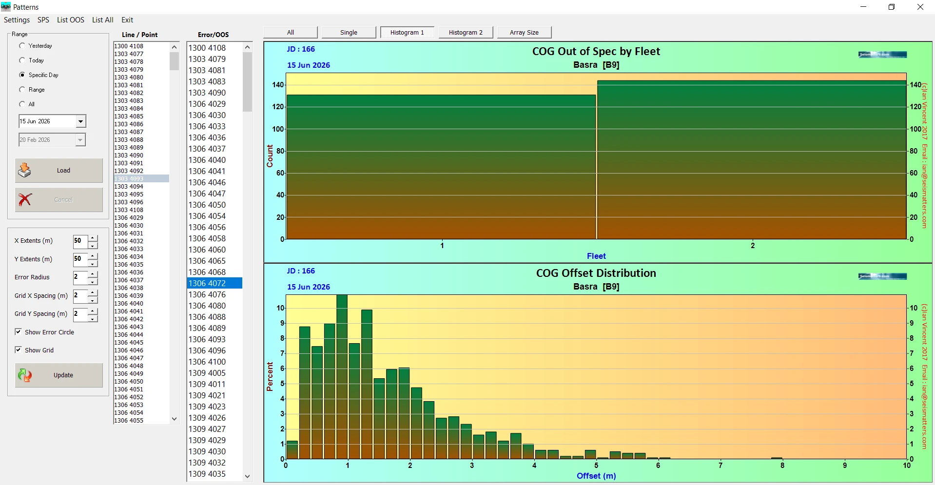
Figure 43. COG QC of the vibrator fleet. Histogram of COG offset distribution.[cite: 1]
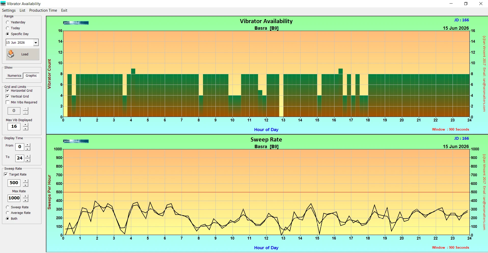
Figure 44. QC of Vibrator availability and the sweep rate on 24h production.[cite: 1]
QC of Sercel Auxiliary traces
There are three (3) auxiliary traces.[cite: 1] Two of them show the autocorrelation of the sweep for each source point during the recording production.[cite: 1] ( The autocorrelation of the pilot sweep is the equivalent T0 in explosive recording ).[cite: 1] Channel Aux2: Autocorrelation of the pilot sweep center at 0.5 second.[cite: 1] Channel Aux3: Autocorrelation of the pilot sweep center at 5.5 second.[cite: 1] ( just for an easier display). Channel Aux1: shows the pilot sweep until six seconds.[cite: 1] (Listening time in our example).[cite: 1]
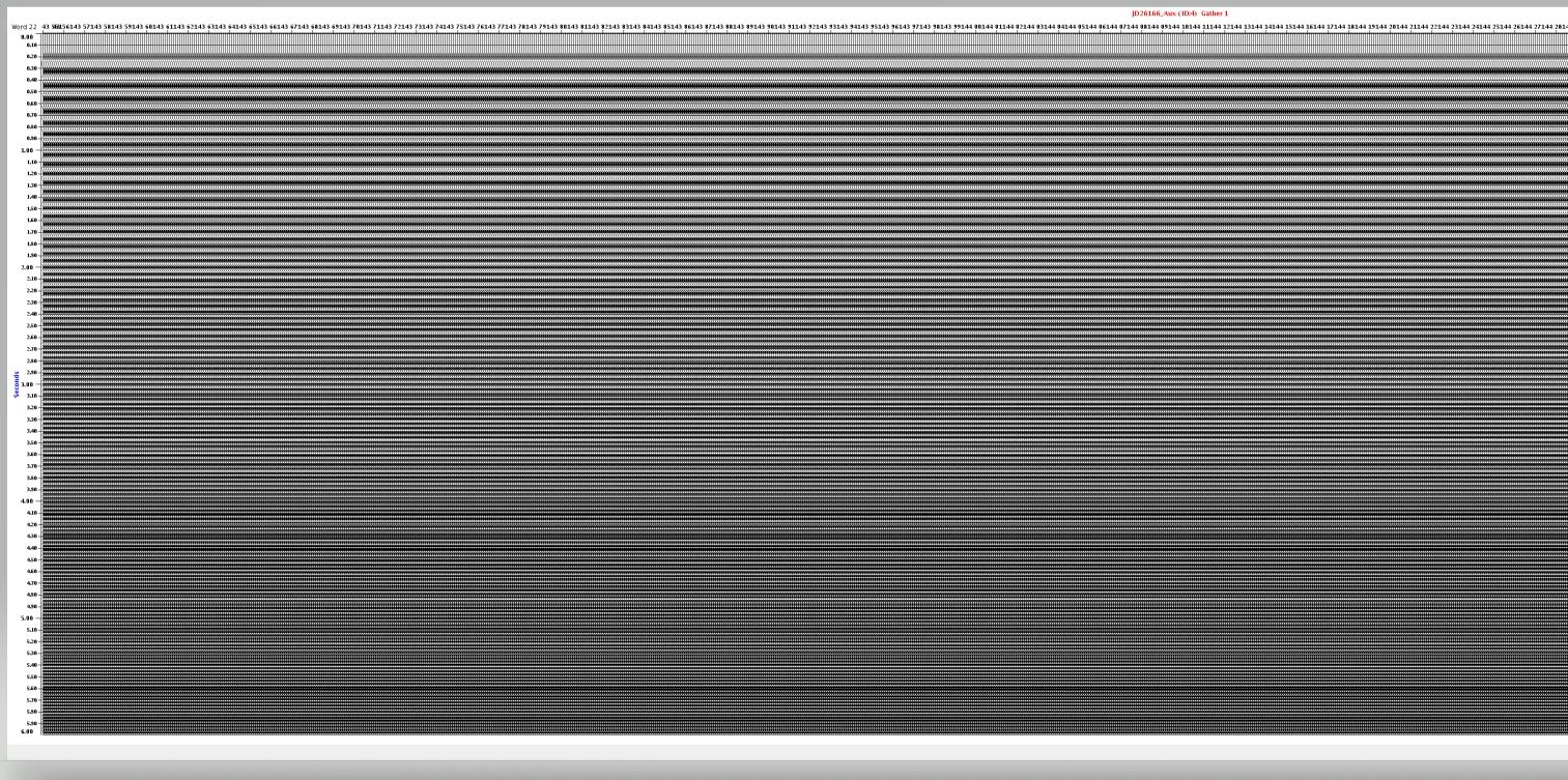
Figure 45. QC of the Auxiliary traces. The pilot Sweep ( until 6 seconds ) for each source point during the recording production.[cite: 1]
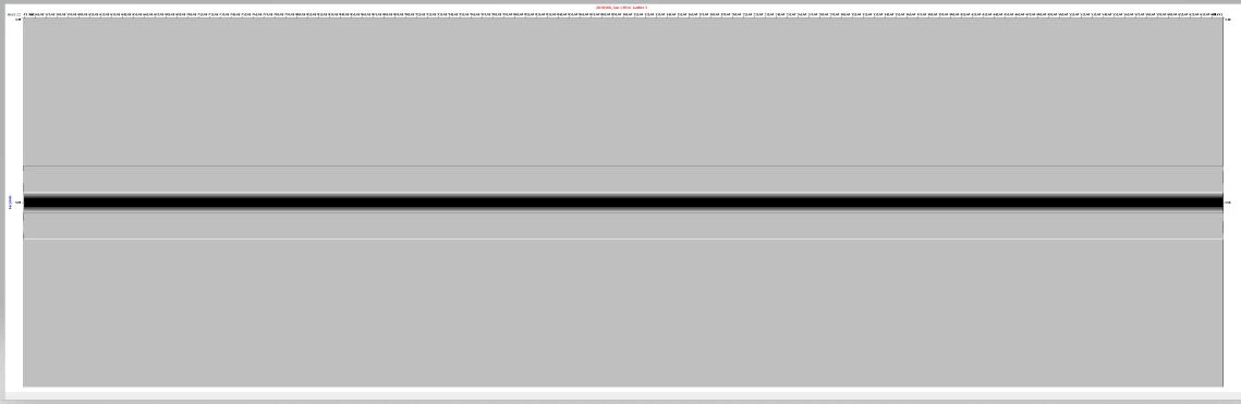
Figure 46. QC of the Auxiliary traces. Channel Aux3: Autocorrelation of the pilot sweep center at 5.5 second for each source point during the recording production.[cite: 1]
The “Magic” of the Correlation Process
Correlation is a mathematical process used to measure the similarity between two signals.[cite: 1] In vibroseis acquisition, the recorded geophone signal is correlated with the pilot sweep.[cite: 1] This process transforms the recorded vibroseis data into a seismic record that is equivalent to the record that would have been obtained using an impulsive source, such as an explosive charge.[cite: 1]
Each seismic reflection can be considered a delayed and attenuated copy of the transmitted pilot sweep (GF).[cite: 1] As the seismic wave travels through the subsurface, reflections are generated at geological interfaces and return to the surface with different travel times.[cite: 1] Consequently, the uncorrelated geophone trace contains many delayed versions of the pilot sweep, mixed with ambient and system noise.[cite: 1]
The purpose of correlation is to identify these delayed sweep “replicas” within the recorded seismic trace.[cite: 1] The correlator continuously compares the pilot sweep with the incoming geophone signal and calculates their degree of similarity at each time sample.[cite: 1] In this example, the seismic data are sampled every 2 ms; therefore, the correlation process is performed every 2 ms throughout the entire acquisition time ( 22 s ).[cite: 1]
Whenever the pilot sweep matches a portion of the recorded seismic trace, the correlation function produces a peak.[cite: 1] The position of this peak indicates the arrival time of a seismic event.[cite: 1] If no similarity exists, the correlation output remains near zero.[cite: 1] The reflection time is determined by measuring the time difference between the correlation peak associated with the reflected event and the peak of the pilot sweep autocorrelation function (T₀), as illustrated in Figure 46.[cite: 1]
Definitions
- * Sweep Length: Duration of the vibrator excitation (pilot sweep). Example: 16 seconds.[cite: 1]
- * Listening Time: Time during which the geophones continue recording after the end of the sweep to capture late-arriving reflections. Example: 6 seconds.[cite: 1]
- * Acquisition Time: Total recording time, equal to sweep length plus the listening time. Example: 16 s + 6 s = 22 seconds.[cite: 1]
- * Correlated Record Length: Length of the seismic record after correlation. For a vibroseis record, this is approximately equal to the listening time. Example: 6 seconds.[cite: 1]
Remarks:
1. The correlation process is performed at every seismic sample (2 ms in this example) throughout the complete 22-second acquisition record.[cite: 1]
2. The length of the correlated seismic record is given by:
Correlated Record Length = Acquisition Time − Sweep Length + 1 Sample[cite: 1]
Therefore:
22 s − 16 s + 1 sample = 6 s + 1 sample[cite: 1]
3. In practical terms, the correlated record length is commonly referred to as the listening time, although mathematically it is equal to the listening time plus one sample.[cite: 1]
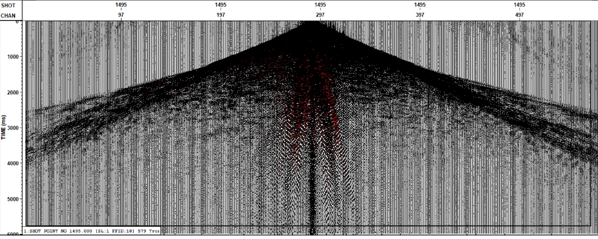
Figure 47. A shot gathers (Correlated record length of 6 s). The seismic data was produced by 16 second-sweep length and listening time of 6 seconds.[cite: 1]