
2.7 Ray Tracing and Elastic Wave Equation Modelling
Seismic modelling helps to evaluate a seismic survey design, especially for complex geologic areas. Interaction with the area's interpreter is paramount to getting a reliable geological model.
Velocity Model Architecture
The velocity to be used in the model is one of the critical factors. For this case, Linear velocity functions V(z) for each layer (geologic formation) were created from well sonic logs over the study area.
The velocity only changes in the vertical direction for each layer. However, due to the complex geology (thrust-belt fold geometry), we also got velocity variations in the horizontal direction. Quality controls applied to the model evaluate key structural components, such as a 3D Geocellular model of the study area, 2D profiles for quality control, dip values, elevation profiles from the interpretation datum, and P-wave velocity values located just above the target layer.
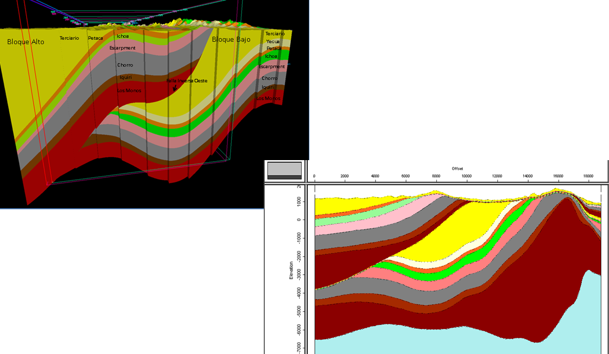
Fig. 1 On the top-left is the 3D Geocellular model of the study area. On the bottom right, a 2D profile in the south of the model for quality control.
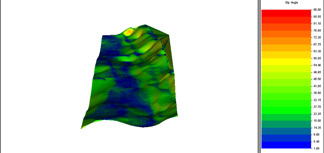
Fig. 2 Quality controls to the model. On the top, dip values for the target layer. On the bottom, P-wave velocity values are just above the target layer.
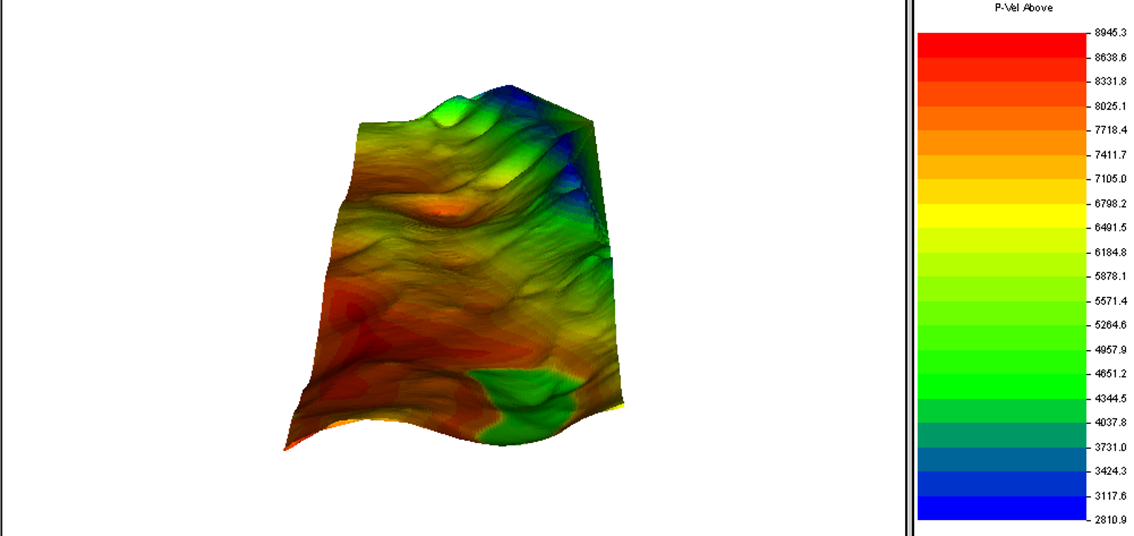
Fig. 3 Quality controls to the model. Elevation of the target layer (From interpretation datum).
Ray Tracing Deliverables
Ray tracing modelling yields several critical design products. A Hit Map provides the exact number of illumination hits for a model target layer. Critical angle analysis and a Maximum Offset Map help define subsurface imaging constraints. The maximum offset maps represent the maximum usable offset before an NMO stretch reaches 30%.
Ray tracing also defines the maximum offset for the target layer, mapping ray paths that emerge from a single subsurface point on the layer and propagate to the surface up to a 30° angle from the vertical. This visualizes the corresponding wavefront at 2.57 seconds. Additionally, a migration aperture map is generated where the migration aperture represents the lateral component of a 30° diffraction traced from the horizon to the surface, with the diffraction angle relative to the vertical.
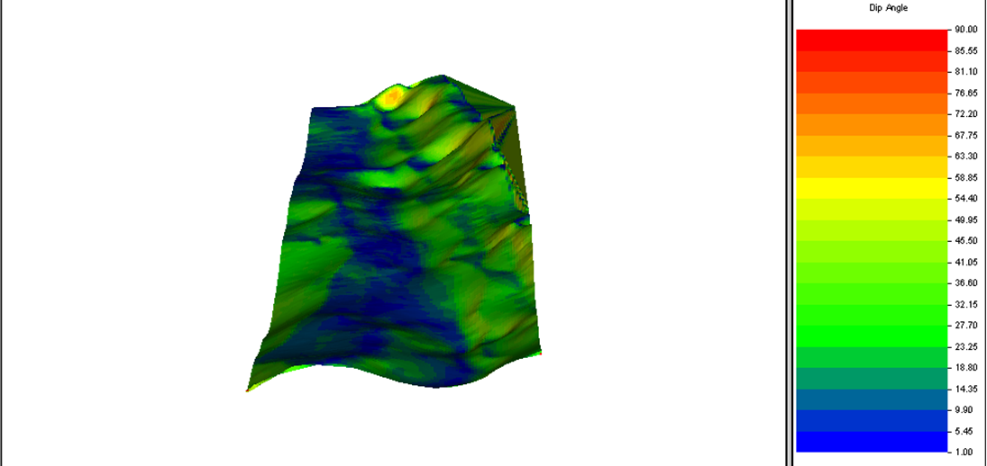
Fig. 4 Ray tracing modelling products. Maximum offset for the target layer. The figure shows the rays coming from one point on the layer (subsurface) to the surface up to a 30° angle from vertical. Also, it shows the wavefront at 2.57 seconds.
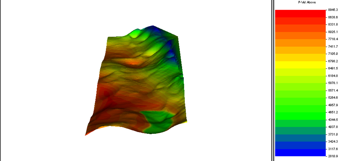
Fig. 5 Ray tracing modelling products. Critical angle analysis.
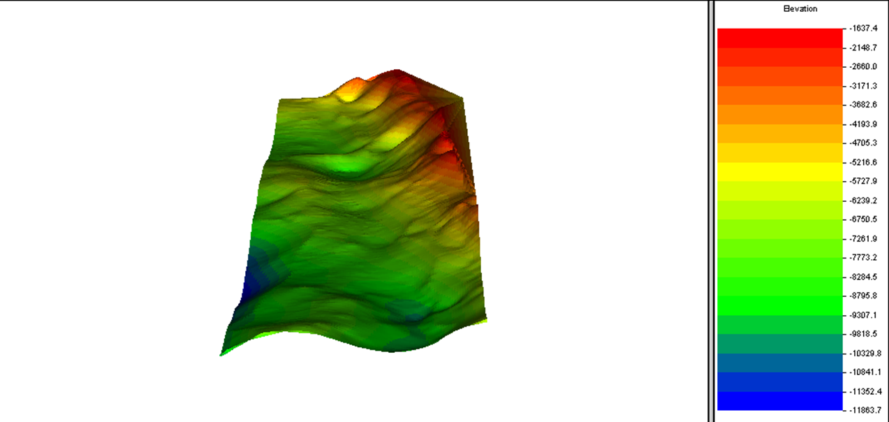
Fig. 6 Ray tracing modelling products. Maximum Offset Map for the target layer. The values represent the maximum usable offset before an NMO stretch reaches 30%.
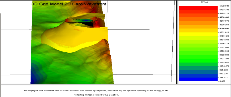
Fig. 7 Ray tracing modelling products. Migration aperture map from ray tracing modelling for the target layer. The migration aperture is the lateral component of a 30° diffraction traced from the horizon to the surface.
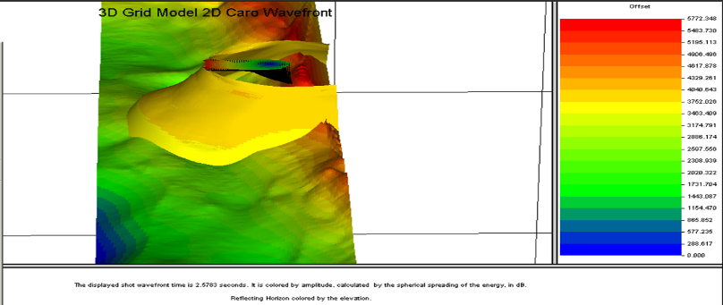
Fig. 8 Ray tracing modelling products. A Hit Map. It gives the number of illumination hits for a model target layer.
Elastic Wave Equation (EWE) Modelling
The EWE modelling produces synthetic shot gathers evaluated in the F-K domain. In a typical scenario where the shot point is in the middle of the 2D model, the gather can be generated with a spatial sampling of ∆G = 15 m and a maximum offset of 12 km, appearing asymmetric due to limitations in the model extension.
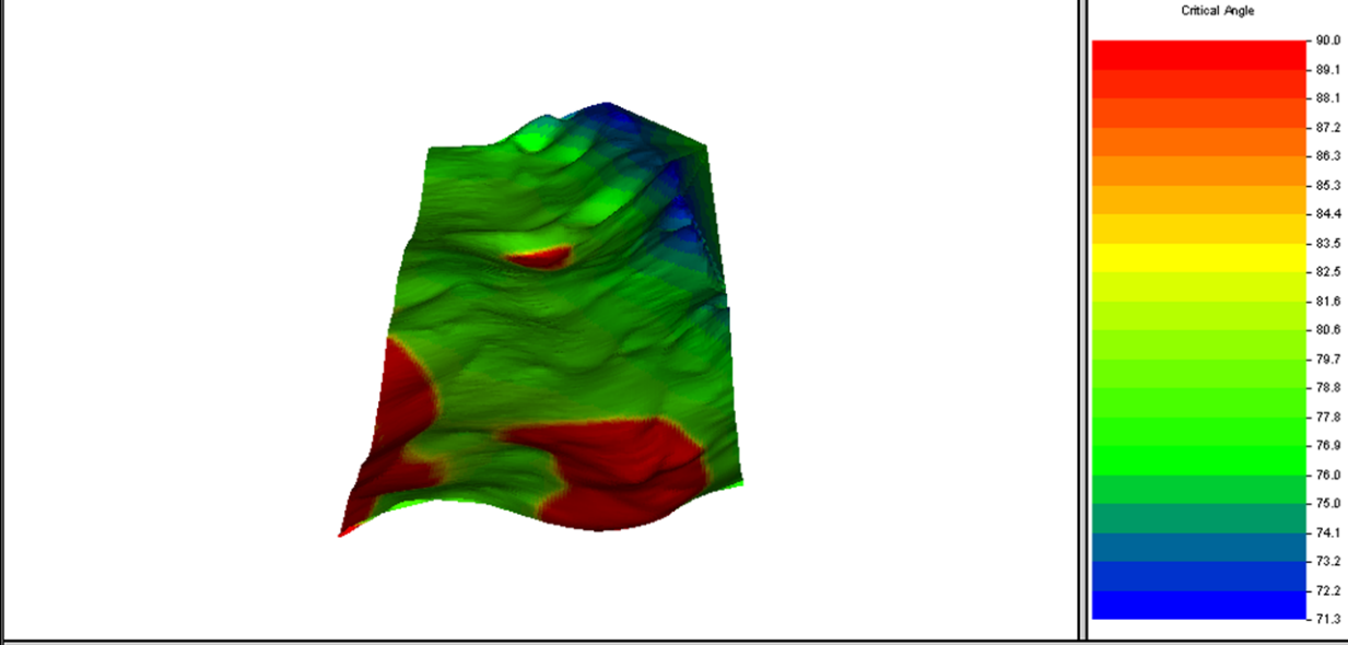
Fig. 9 A synthetic shot-gather using Elastic Wave Equation (EWE) modelling. The shot point is in the middle of the 2D model. The gather was generated with a spatial sampling of ∆G = 15 m and a maximum offset of 12 km.
By modeling with different receiver station intervals (∆G), the spatial sampling thresholds can be explicitly evaluated. For a ∆G = 10m, the F-K analysis shows no spatial aliasing for all wavelengths, verifying the full wave sampling method.
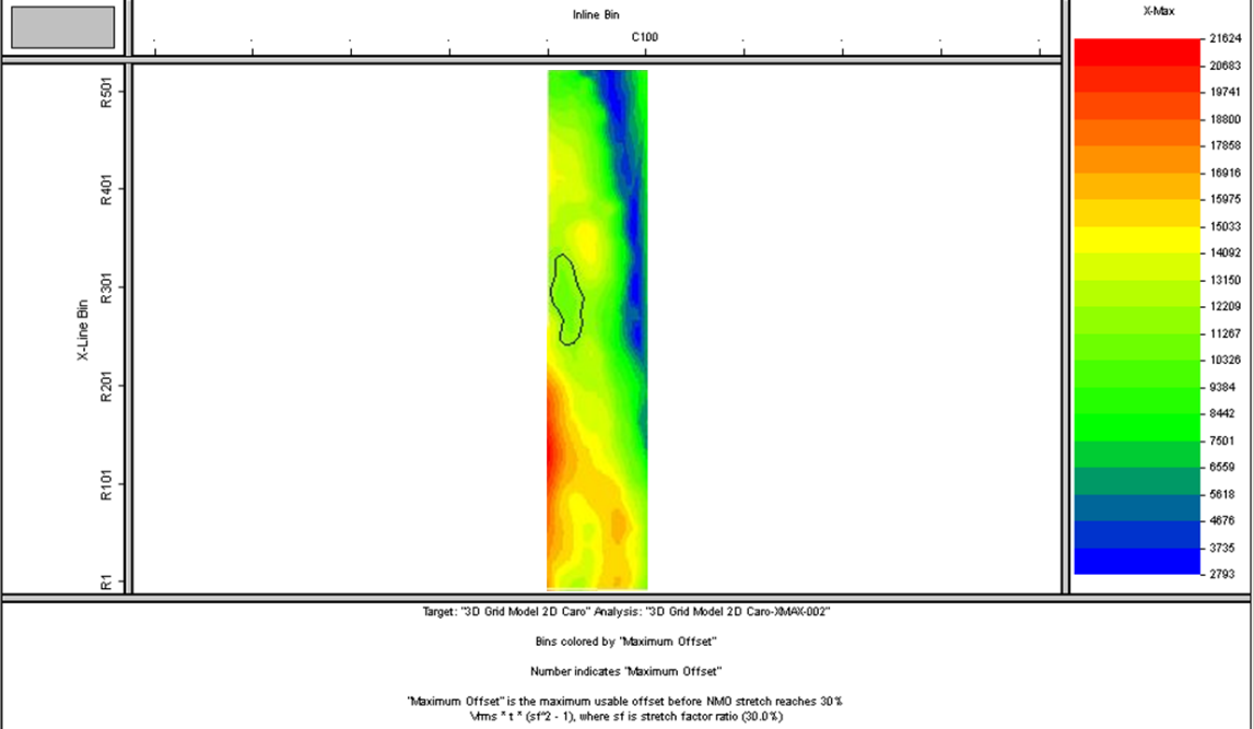
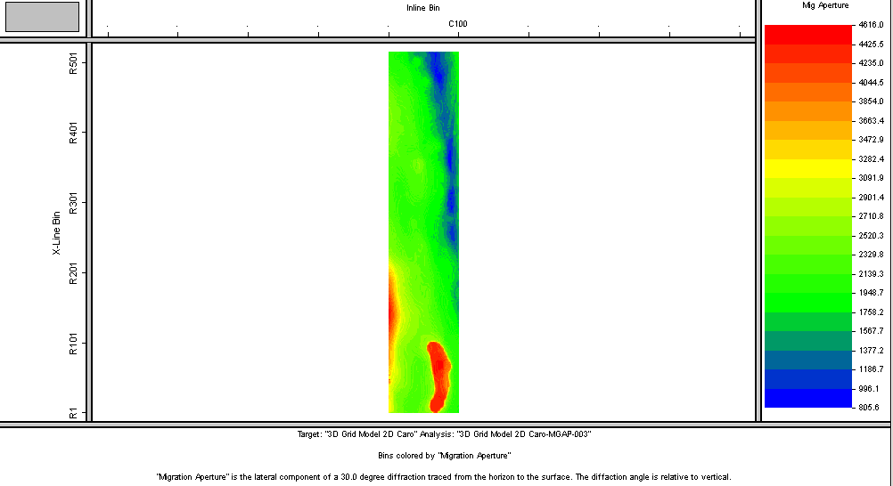
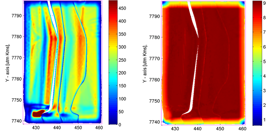
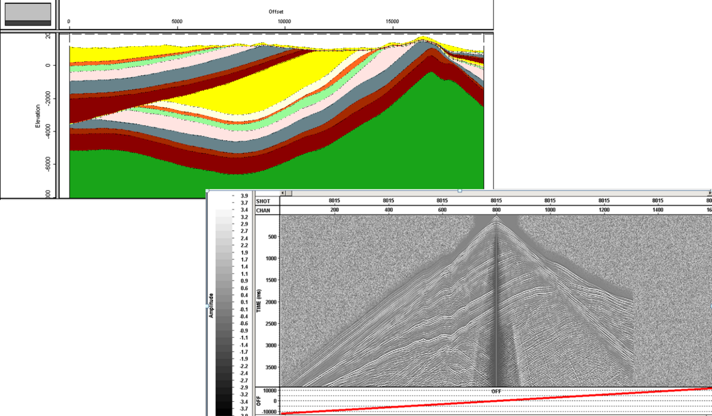
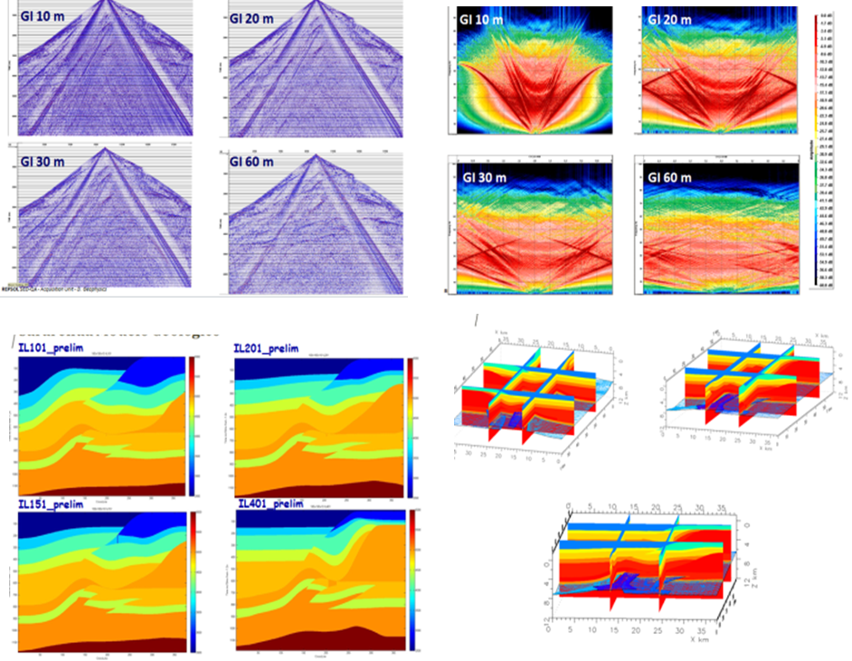
Fig. 10 Synthetic shot-gathers from EWE Modelling with different receiver station intervals (∆G). The EWE modelling produces synthetic shot gathers evaluated in the F-K domain.
If your computer power is big enough and you have plenty of time for designing, you could produce a complete synthetic seismic survey and then process it to evaluate the outcome from a specific survey design.